Pathtracer
UC Berkeley - Summer 2020
Part 1: Overview
For my Computer Graphics class at UC Berkeley, I implemented a ray tracer that renders realistic materials by mapping light rays through a scene. In the first part of the project, I generated rays and wrote functions to check for ray-object intersections so that my program would know when light has hit a surface. Then I implemented a bounding volume hierarchy (BVH) algorithm that optimizes ray tracing. The algorithm uses a binary tree to group primitives into bounding boxes so that a ray will only have to be tested against a few primitives in the bounding box that it hits instead of having to test against all primitives in a scene. I then worked on implementing different kinds of lighting using Monte Carlo integration: direct illumination and global illumination. The last part of the project was implementing adaptive sampling, which allows for renders that use a large amount of samples-per-pixel while still maintaining an efficient computation time.
Part 1.1: Ray Generation and Scene Intersection
When rendering an image, ray generation is used to send rays through a pixel and into an image's world space to determine the radiance in that pixel. The radiance affects what color the pixel will take on in the image after using a Monte Carlo estimate of random rays in one pixel. For a given pixel (x, y) in the image space, a random sample within (x, y) and (x + 1, y + 1) is converted to a ray in camera space using a (0, 0, 0) origin and a field of view transformation to turn the sample's 2D coordinates into the ray's direction vector which will be (sample x - 0.5 * 2 * tan(0.5 * hFov), sample y - 0.5 * 2 * tan(0.5 * vFov), -1). This camera ray points down the -z axis by convention. The camera space ray is then rotated and translated to world view using a rotation matrix and a world view position origin. Once the ray is in world space, the ray can be tested against objects, like triangles and spheres, in the world space scene to see if it intersects any objects. To see if the ray itersects the object, the Moller Trumbore algorithm can be used for triangles and the roots of the (o + t*d - c)2 - R2 = 0 equation can be used for a sphere. If the ray intersects with the object, the time t and the surface normal of the intersection point can be recorded to be used for the average shading and radiance color values at the pixel that the ray originally went through.
The triangle intersection algorithm that I used is the Moller Trumbore algorithm. The algorithm uses the ray equation and barycentric coordinates to determine whether a ray intersects a triangle, and if it does, at what time t the intersection occurs. The algorithm's main equation is o + td = (1 - b1 - b2)P0 + b1P2 + b2P2. The left hand side of the equal sign is the ray equation where o is the origin vector, t is the time, and d is the direction vector. P0, P1, and P2 are the coordinates of the vertices of the triangle, and b1, b2, and b0 = 1 - b1 - b2 are the barycentric coordinates. To solve for the values [t b1 b2], the various vertices and ray origin and direction are used in a series of cross products, dot products, subtraction, etc shown below.
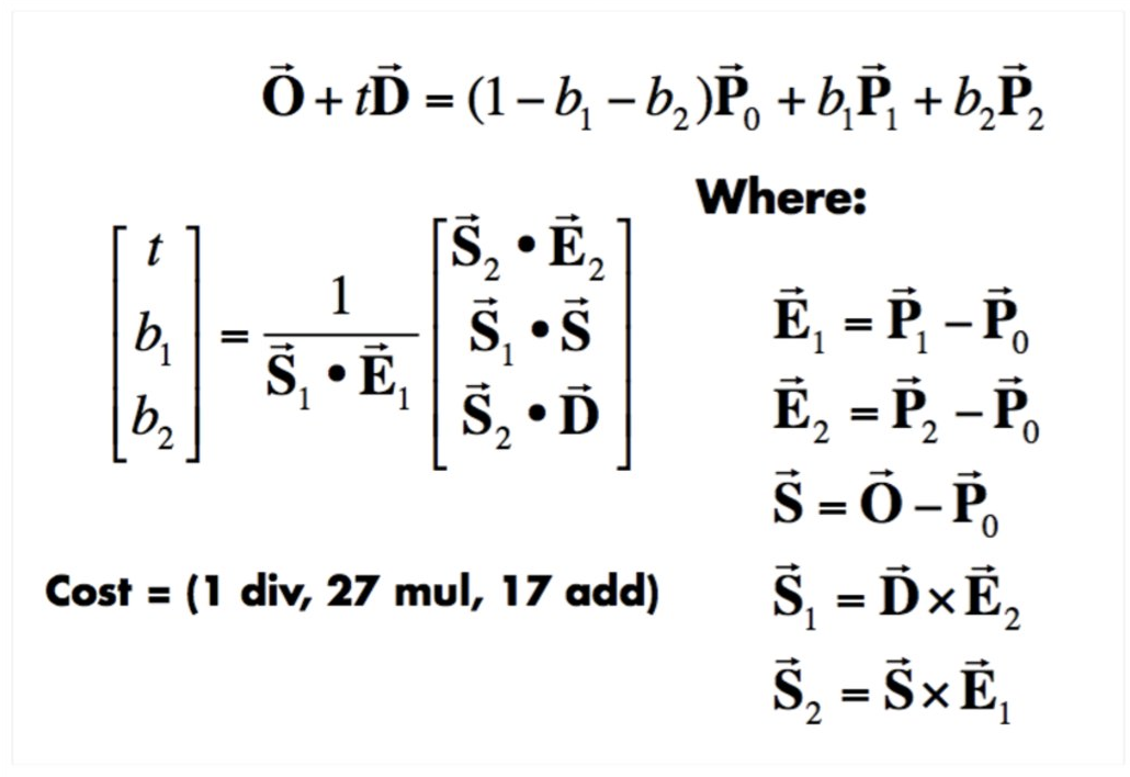
After solving for the [t b1 b2] values, if the time t is > 0 and is within the min and max t of the ray (to ensure this is a valid intersection), and the barycentric coordinates are all within [0, 1], then the t is the time of the ray intersecting the triangle. The surface normal of the point of intersection can be found using the normals of the vertices of the triangle and the barycentric coordinates, and this normal can be used for shading of the pixel that the ray goes through in the image.
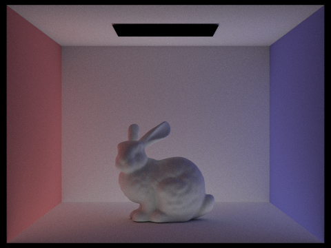
Empty Cornell box with normal shading.
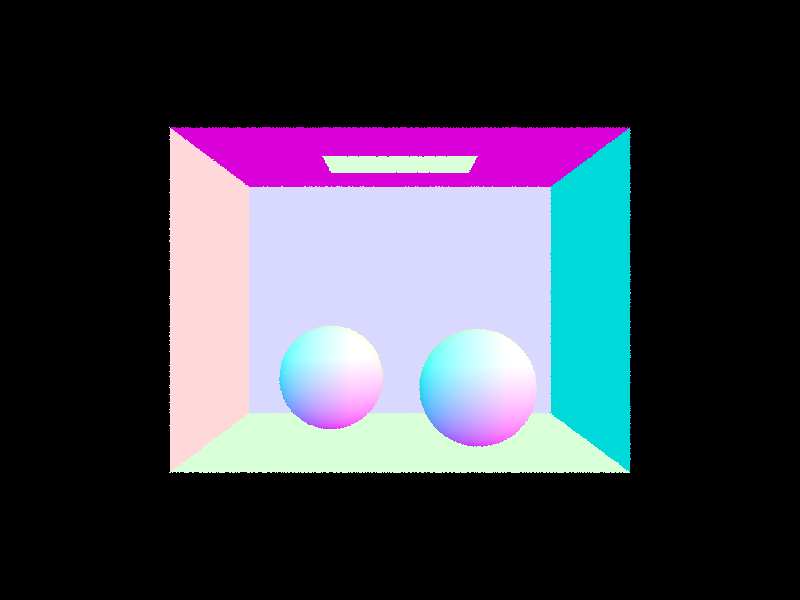
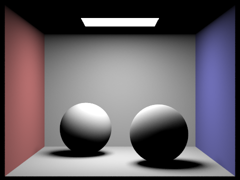
Cornell box with spheres and normal shading.
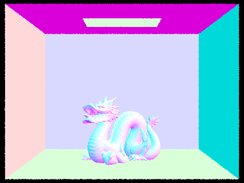
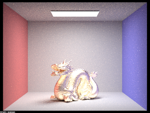
Cornell box with dragon and normal shading.
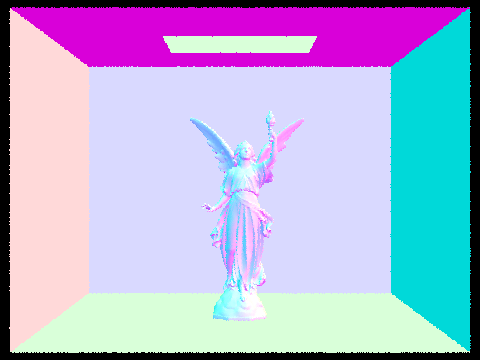
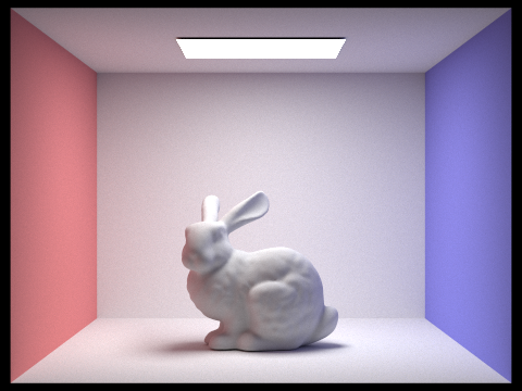
Cornell box with Lucy and normal shading.
Part 1.2: Bounding Volume Hierarchy
The bounding volume hierarchy (BVH) construction algorithm splits primitives within a scene into a tree structure by grouping the primitives into "bounding boxes." The tree structure is a binary tree where the leaves of the tree hold lists of primitives whose centroids fall within the bounding box of the leaf. The leaves connect to internal nodes that don't hold primitives, but have bounding boxes that encase the bounding boxes of its child nodes. The algorithm groups primitives based on a heuristic that splits an axis of the scene and groups the primitives along the axis into a left group or right group. To begin my algorithm, I built the bounding box that contains all of the current primitives and another bounding box that contains the centroids of the primitives. Then I checked to see if the current node/level of the BVH has less than max_leaf_size number of primitives in it. If it has less, then the node is a leaf and will contain all of the primitives in its bounding box. If it has more than the max size, then I use a heuristic to split the primitives into a left and right child to recurse on. By splitting the primitives up into various bounding boxes, ray tracing can be accelerated because a ray can quickly reject a branch of the BVH tree if it doesn't intersect with the outer bounding box of the primitives within the branch. This way, no time is wasted testing ray intersections on primitives that are no where close to the ray.
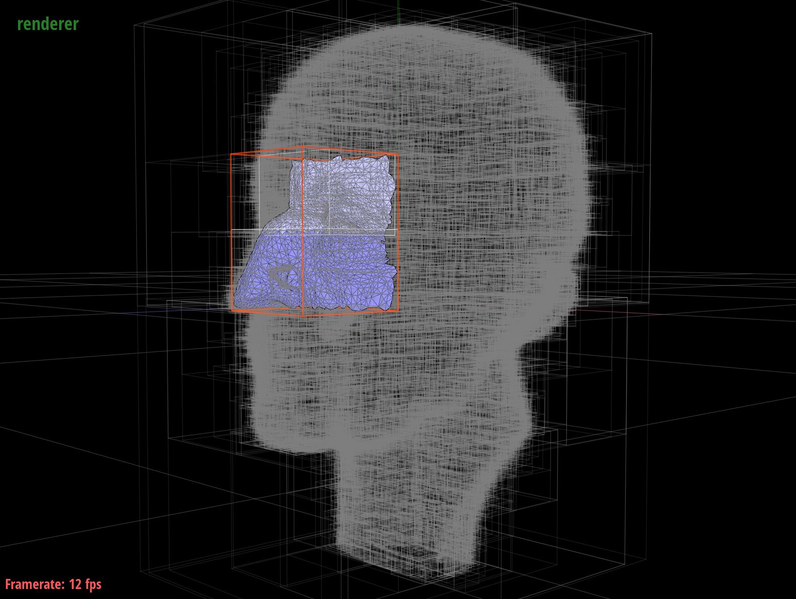
The bounding boxes of 2 internal branches of the BVH of maxplanck.dae's geometry can be seen here.
I chose to split along the longest axis of the primitive centroid bounding box and group primitives into the left or right group based on their centroid's position on either side of the midpoint of the centroid bounding box's splitting axis. I originally chose the longest axis of the node's bounding box and used the midpoint as the split point, not using a centroid based bounding box, but I ran into problems where the split point would not be in the middle of the primitives. One group would get all the primitives, while the other would be empty very early on. I tried to fix this issue using quicksort on the group that got all the primitives and splitting the sorted vector in half, but I found that my quicksort would work for some large dae files, but not others. After inspecting the CBLucy.dae mesh, I realized that maybe the longest axis of the bounding box is the longest distance wise, but the actual spread of the centroids of the primitives may not be longest on this axis. I then switched to the centroid bounding box midpoint heuristic, and this fixed my problem of uneven splitting.
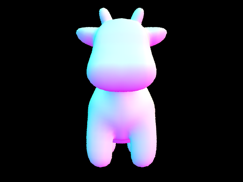
cow.dae with normal shading
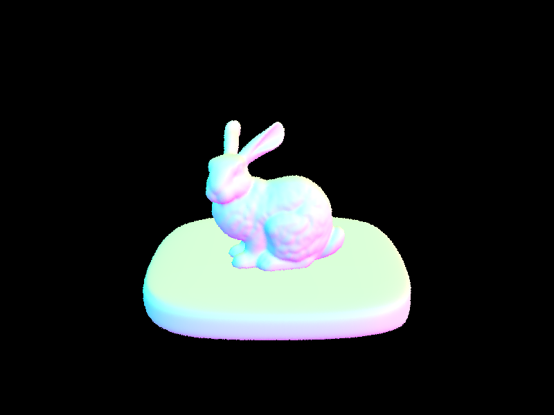
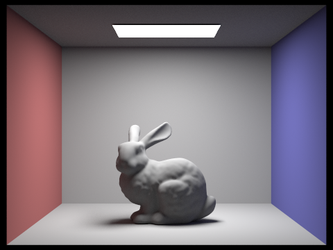
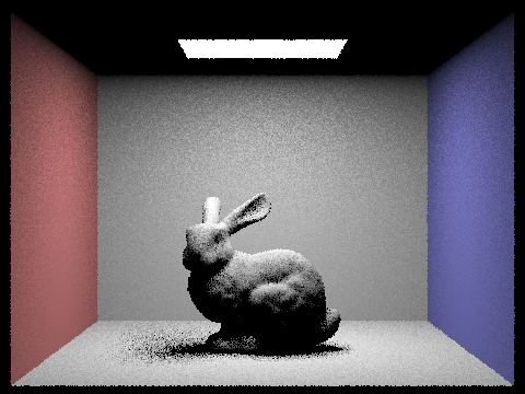
bunny.dae with normal shading
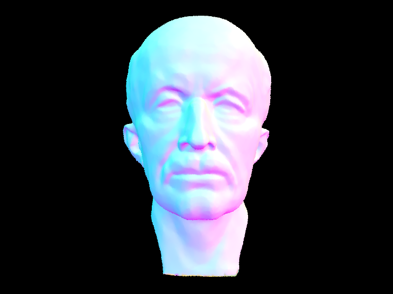
maxplanck.dae with normal shading
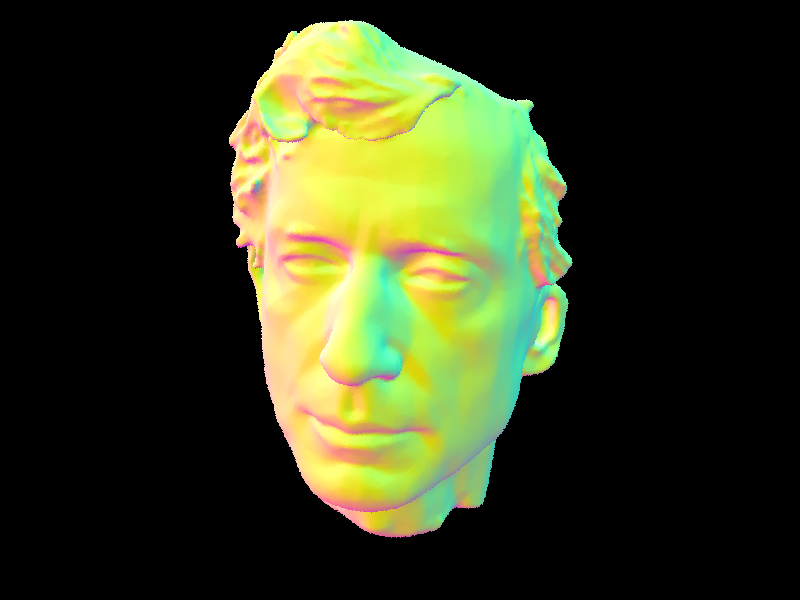
peter.dae with normal shading
The meshedit/cow.dae mesh took 32.0146s without BVH acceleration, but only took 0.1033s with BVH acceleration. The sky/bunny.dae took 253.2246s without BVH acceleration, but only took 0.1066s with BVH acceleration. The meshedit/maxplanck.dae took 358.7527s without BVH acceleration, but only took 0.1578s with BVH acceleration. The meshedit/peter.dae took 286.3262s without BVH acceleration, but only took 0.1410s with BVH acceleration. These four geometries of varying complexities are 6862x faster than the non-accelerated BVH when averaged together. This impressive acceleration is thanks to the BVH because large amounts of computation can be skipped when calculating ray intersections since a single ray will only intersect with a few primitives in a leaf of the BVH, and testing all of the primitives in the entire scene is a waste of time and energy.
Part 1.3: Direct Illumination
The uniform hemisphere sampling version of the direct lighting function calculates irradiance at uniform sample angles of a hemisphere for pixels in an image. For each pixel, the uniform hemisphere samples are used as the directions of rays pointing from the pixel into the image's scene in world space. If this ray built from the sample intersects with a primitive in the scene, the reflection equation of the surface at the intersection (which multiples the bsdf of the surface, the radiance of the intersection object, and a cosine of the sample direction) weighted by 1 / 2 * PI (because of the uniform hemisphere) will be added to the estimate of the irradiance of the pixel. However, for most of these uniform samples, the radiance coming into the pixel from the uniform hemisphere sample direction is zero because the chance that the sample is coming from a light source is very small, and we only care about direct light. Uniform hemisphere sampling tends to be noisy because most samples don't have any incoming radiance, and therefore the irradiance going out of the pixel in the sample direction doesn't have any light.
The importance sampling version of the direct lighting function calculates irradiance at pixels in an image by directly sampling light sources. Directly sampling light sources reduces the noise in the output image because all of the sample rays that don't intersect anything when going from a pixel to the light source have non-zero radiance, and therefore will be in a direct light. Instead of choosing uniform samples, samples are taken on light sources using a pdf that weights the directions pointing at a light source heavily. Using this sample that will be more likely to have a non-zero radiance, the same reflection equation as hemisphere sampling is used to get an estimate of radiance.
CBbunny.dae rendered with uniform hemisphere sampling.

CBbunny.dae rendered with importance light sampling.
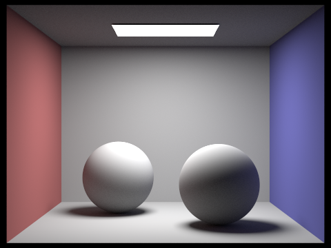
CBspheres_lambertian.dae rendered with uniform hemisphere sampling.
CBspheres_lambertian.dae rendered with importance light sampling.
When there are more samples per area light (light rays), the soft shadows underneath the bunny become less noisy because more radiance samples that point at the light will be included and weighted heavily in the estimate of irradiance for the pixels that are on the ground close to the bunny.

CBbunny.dae with 1 light ray.
CBbunny.dae with 4 light rays.

CBbunny.dae with 16 light rays.

CBbunny.dae with 64 light rays.
Overall, uniform hemisphere sampling is more noisy than importance sampling due to the greater chance than a sample ray will not point at a light source. If a sample ray doesn't point at a light source, then there is no radiance along the ray and therefore no irradiance at the pixel where the ray originated. When estimating direct light, importance sampling does a better job because the sample rays that are used for the estimation of irradiance actually point at the light and will have direct lighting to use for the irradiance unless that ray intersects with a primitive in the scene.
Part 1.4: Global Illumination
For my implementation of global illumination, I recursively follow rays from the camera into world space to track how light bounced around the scene and ended up at the camera. Using this technique, indirect light that has reflected off of non-light objects can show up in the rendered image in addition to the direct lighting from light sources. To begin the algorithm, I check which bounce the current ray is on. If it's zero, then there is no bounce and zero radiance is returned (which would only be pixels that are the light source). If the ray is on the first bounce, then the direct lighting one bounce function is called. If the ray is on a bounce > 1, then a new ray is built from the current point and given a sample direction using a pdf. This new ray is tracked in the world scene and its reflection equation is calculated as usual except that the at_least_one_bounce/indirect lighting function is called recursively in the reflection equation to get a value for the radiance L. The intersection point of the ray will become the next point to sample in the recursive call. Thus, the recursion tracks light through the scene by bouncing along with the ray and estimating radiance at each new surface the sample ray intersects and reflects off of. To stop the recursion, I use a coin flip of probability 0.65 for Russian Roulette termination and also a max ray depth to ensure there are no infinite loops or really long computation times. The estimations for the radiance calculation are normalized by the sample pdfs used and the 0.65 Russian Roulette probability so that later bounces are not weighted as heavily since they do not add as much information to the radiance calculation as earlier bounces.
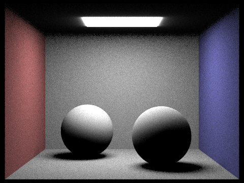
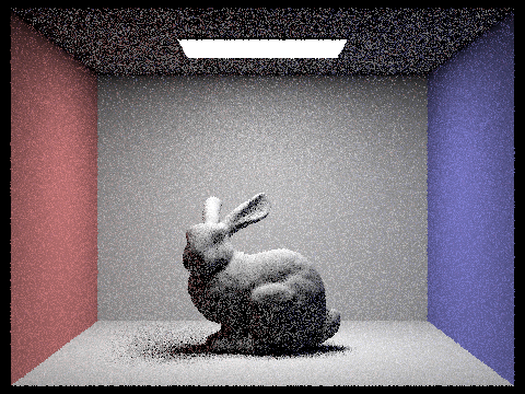
CBspheres_lambertian.dae rendered with global illumination, 1024 samples-per-pixel, 16 light rays-per-pixel, and max 5 bounces.

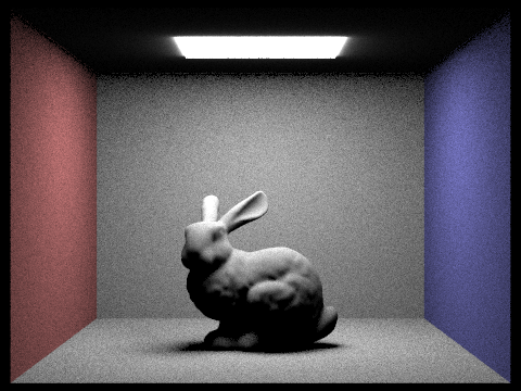
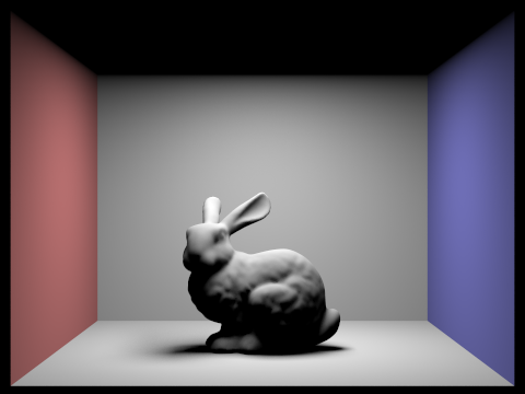
CBbunny.dae rendered with global illumination, 1024 samples-per-pixel, 16 light rays-per-pixel, and max 5 bounces.
CBbunny.dae with only direct lighting.
CBbunny.dae with only indirect lighting.
CBbunny.dae with max ray depth of 0.

CBbunny.dae with max ray depth of 1.

CBbunny.dae with max ray depth of 2.

CBbunny.dae with max ray depth of 3.

CBbunny.dae with max ray depth of 100.
CBbunny.dae with 1 sample-per-pixel.

CBbunny.dae with 2 samples-per-pixel.

CBbunny.dae with 4 sample-per-pixel.

CBbunny.dae with 8 samples-per-pixel.

CBbunny.dae with 16 samples-per-pixel.

CBbunny.dae with 64 samples-per-pixel.
CBbunny.dae with 1024 samples-per-pixel.
Part 1.5: Adaptive Sampling
To implement adaptive sampling, I first kept running totals of each sample's illuminance and squared illuminace so that I could compute the mean and variance of all the current pixel's samples so far. If the current sample modulo the samplePerBatch number is 0, then I would compute the variable I using the mean and variance formulas and test I against maxTolerance * the mean. If I was less than the maxTolerance * the mean, then the pixel has converged because a small I means the pixel doesn't have a large variance (not much variety in the samples' estimated colors) or there have been a lot of samples so the current estimation is sufficient based on a 95% confidence interval. When I passes the tolerance check, I break out of the for loop and then update the pixel's estimation as the sum of its estimated radiance divided by the number of samples taken before convergence (or the max number of samples if the pixel didn't converge). This allows for rendering with a large amount of samples-per-pixel, but cuts down on computation time for different parts of the image that has pixels that converge faster and don't need as many samples.
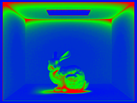
CBbunny.dae adaptive sampling rate.
CBbunny.dae rendered with adaptive sampling, global illumination, 4096 samples-per-pixel, 128 pixel batches, 1 light ray per-pixel, and 6 max ray depth.
Part 2: Overview
For the second part of the project, I added new materials to the pathtracer so that objects with mirror, glass, or microfacet surfaces could be rendered. I implemented different BRDFs for each of the three materials that use specular reflection, refraction, and normal distributions in order to imitate how light rays bounce off the surface of mirror and glossy materials in one direction or one general direction. This is different than the diffuse material BRDF in part one that reflects light equally in all directions.
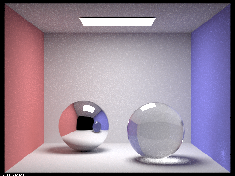
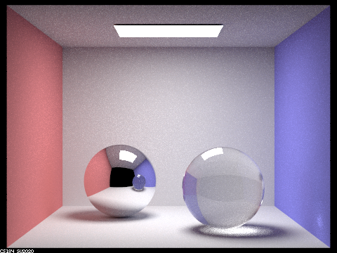
Part 2.1: Mirror and Glass Materials
When rendering mirror and glass materials like in CBspheres.dae with an area light, light effects that resemble real life start to show up as a ray is traced through multiple bounces around a scene. This is because mirrors use specular reflection which requires 2 bounces and glass uses reflection but also refraction of light through its surface, which uses 3 bounces. In the images below, the image with ray depth of 0 only shows the area light because no rays are traced out of the light source. In the image with ray depth 1, the pixels of the image that can reach the light source through an uninterrupted ray are lit up because they are in direct light from the light source. The direct reflection of the light source on both spheres that looks like a white, curved rectangle shows the beginning of the reflection of the mirror and glass spheres. In the image with ray depth 2, the mirror sphere now shows a reflection of the Cornell Box with direct lighting because rays can bounce once on the surface of the sphere and then reflect/bounce again off the sphere to get the mirror effect. Since the light that is reflecting off the sphere is direct light from the ray of the first bounce, the mirrored picture on the ball doesn't show the lighting effects of the second bounce like the non-black ceiling. The glass sphere also shows some reflections, but the refraction doesn't fully work yet because refraction requires that a ray of light "bounces" once on the surface of the sphere, "bounces" through the sphere to the other side based on the refraction direction, and then has to "bounce again" out of the sphere and onto another surface or to the camera to get the full refraction effect. In the image with depth 3 and above, the refraction process can complete because now 3 bounces of light are allowed. Light from the light source can now refract fully through the sphere, and the light below the glass sphere in the middle of the sphere's shadow has gotten brighter because more light can transmit through the ball with higher numbers of max ray depths. In the images with depth 4 and higher, a caustic can be seen to the right of the glass ball. The caustic effect shows up when a light reflects or refracts off a surface and then hits a diffuse surface before hitting the camera. The caustic only shows up when max ray depth is at least 4 because light must bounce once on the surface of the glass sphere, bounce through the sphere to the other side, bounce out of the sphere to the diffuse surface (the wall), and then bounce off the diffuse surface to the camera or another surface.

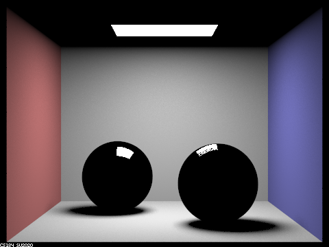
CBspheres.dae with depth 0.
CBspheres.dae with depth 1.
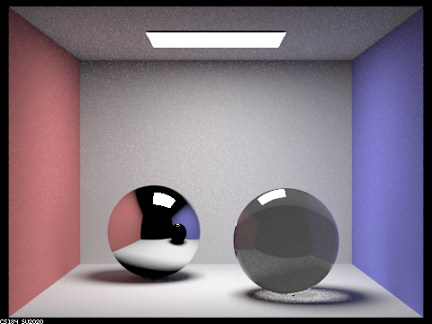
CBspheres.dae with depth 2.
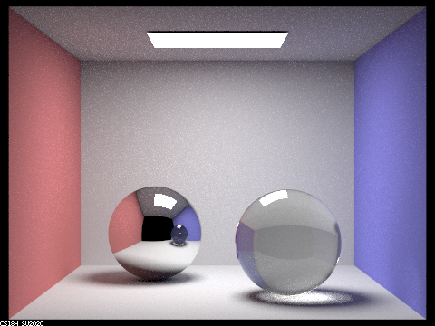
CBspheres.dae with depth 3.

CBspheres.dae with depth 4.
CBspheres.dae with depth 5.
CBspheres.dae with depth 100.
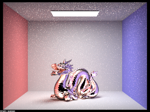
Part 2.2: Microfacet Material
For this part, I implemented a BRDF that uses the Beckmann NDF, Fresnel terms, and importance sampling to compute the color of sample rays that hit a microfacet surface compromised of small specular elements. The dragons below have different alpha values that determine the roughness of the microfacet surface. In the first image, the alpha is small, 0.005, so the surface of the dragon is glossier. This is because the roughness is low, so the macro surface of the dragon is smoother, similar to a mirror, that reflects light in the general direction of the reflection angle. The next image with an alpha of 0.05 is also quite glossy and reflects light similarly to a mirror, but this dragon is slightly brighter because now light from the area light source is being reflected in more directions than the image with the smaller alpha due to the rougher surface. The greater alpha gets, the more diffuse the macro surface of the dragon, so light will reflect off the microfacet surface in less concentrated directions as alpha gets bigger. In the image with alpha of 0.25, the surface of the dragon has become rougher and the dragon has lost some of its glossy shine. The dragon looks more matte because the roughness of the surface has increased and light is reflecting off of the more uneven microfacets in less concentrated directions. The last image with an alpha of 0.5 is the most diffuse because the roughness variable is the highest. This dragon is not glossy and instead looks matte due to light reflecting off the microfacets in all directions instead of a general direction.
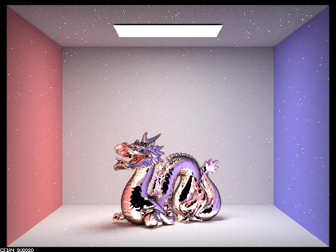
Microfacet gold dragon with 0.005 alpha, 128 samples-per-pixel, 1 sample-per-light, max ray depth 5.
Microfacet gold dragon with 0.05 alpha, 128 samples-per-pixel, 1 sample-per-light, max ray depth 5.
Microfacet gold dragon with 0.25 alpha, 128 samples-per-pixel, 1 sample-per-light, max ray depth 5.
Microfacet gold dragon with 0.5 alpha, 128 samples-per-pixel, 1 sample-per-light, max ray depth 5.
The bunny on the left uses cosine hemisphere sampling and is slightly noisier and darker than the bunny that uses importance sampling. This is because cosine hemisphere sampling picks samples evenly over a hemisphere, and doesn't give any priority to samples that have a greater effect on the colors and lighting of the image. Since microfacets are using the Beckmann NDF, the importance sampling needs to match the distribution of the normals instead of being uniform like the cosine hemisphere sampling. By using importance sampling, samples that add more to the image are given more weight, so the importance sampled bunny is less noisy, brighter, and shinier.
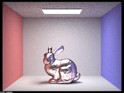
Microfacet copper bunny with cosine hemisphere sampling and 0.5 alpha, 64 samples-per-pixel, 1 sample-per-light, max ray depth 5.
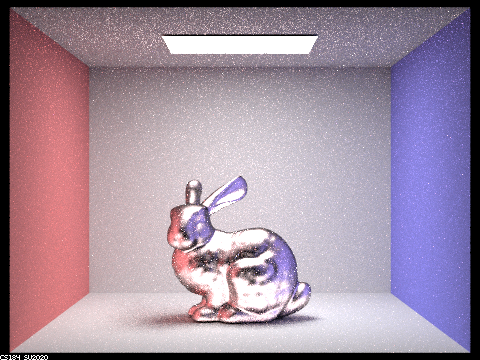
Microfacet copper bunny with importance sampling and 0.5 alpha, 64 samples-per-pixel, 1 sample-per-light, max ray depth 5.
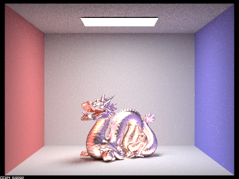
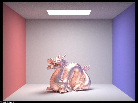
For my different material, I changed the dragon's material from gold to silver. Silver's indices of refraction for the rgb wavelength values are eta: 0.059193, 0.059881, and 0.047366, and k: 4.1283, 3.5892, and 2.8132.
Microfacet silver dragon with new eta and k, and alpha = 0.5

